Animated 3D plot in spherical coordinates with gnuplot
Published:
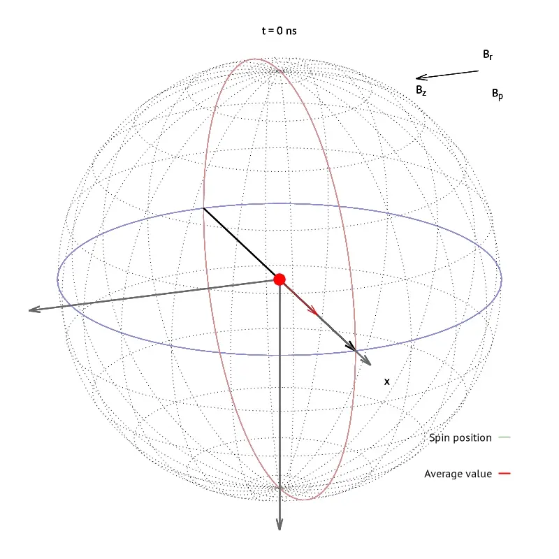
I am working on a physics experiment that involves muons that are stored in a magnetic field and are traveling along circular orbits. Their motion inside the magnetic field is quite complex and involves oscillations with different periods – essentially they are like a spinning top, but instead of precessing around only one axis, they can precess around three.
What I am interested in is to track the spin of the muons through time and in
order to visualize things better I wanted to have an animated 3D plot of the
vector of the spin as the muons experience the changing magnetic field. My
favorite plotting tool for 3D graphs is gnuplot.
The code to generate this plot is a bit large and messy, but it may be useful to someone so I’m posting it here:
# Initial spin vector
Sx = -0.0
Sy = -1.0
Sz = -0.0

# Transform to spherical coordinates
phi_0 = atan2(Sx, Sy) # rad
theta_0 = atan2(sqrt(Sx**2+Sy**2), Sz)-pi/2 # rad

# Spin motion equations
Eex = 0.05
e_z = 2.956e-3*(1.0+Eex) # rad/ns
om_z = 2*pi/42000*Eex/0.05  # rad/ns
omega = 0.03264 # rad/ns

f(x) = (191.49*(Eex) + 178.05*0.06/27.94/omega)*(cos(omega*x))
l(x) = -(((sin(omega*x+phi_0)))*81.75e-3/omega)
p(x) =  phi_0 -om_z*x
if (om_z != 0) {
    e(x) = -e_z/om_z*sin(p(x))
} else {
    e(x) = e_z*x*cos(phi_0)
}
c =    (f(0))*sin(p(0)) + l(0)*cos(p(0)) + e(0)
g(x) = (f(x))*sin(p(x)) + l(x)*cos(p(x)) + e(x) + theta_0 * 1e6 - c
# End of spin motion equations

# Plotting
set key samplen 1 height 5 bottom
set view 70, 340, 1.6, 1.6
set view equal xyz
set parametric
unset xtics
unset ytics
unset ztics
set border 0
set xlabel 'p'
set ylabel 'z'
set isosamples 12
set xyplane -0.5
set grid x y
set xrange [-1:1]
set yrange [-1:1]
set zrange [-1:1]
set urange [0:2*pi]
set vrange [-pi:pi]


phi(x) = (g(x) - theta_0*1e6 + c) / 20 + theta_0 - c / 1e6
the(x) = p(x) + f(x) * sin(phi(x)) / 20
av_the(x) = p(x)
av_phi(x) = e(x) / 20

av_x(u, v) = v*cos(av_the(u))*sin(av_phi(u))
av_y(u, v) = v*cos(av_the(u))*cos(av_phi(u))
av_z(u, v) = v*sin(av_the(u))

fx(u,v) = v*cos(the(u))*sin(phi(u))
fy(u,v) = v*cos(the(u))*cos(phi(u))
fz(u,v) = v*sin(the(u))

# Parametric functions for the sphere
r = 1.0
sx(u,v) = r*cos(u)*sin(v)
sy(u,v) = r*cos(u)*cos(v)
sz(u,v) = r*sin(u)

# Plot axis vectors
set arrow 2 from 0,0,0 to 0,-1.2,0 lc rgb 'gray40' lw 2 back
set arrow 5 from 0,0,0 to -1.2,0,0 lc rgb 'gray40' lw 2 back
set arrow 6 from 0,0,0 to 0,0,-1.2 lc rgb 'gray40' lw 2 back

# Plot magnetic fields in the top right corner
o = 0.3
o0 = 1.5
set arrow 7 from o0,o0,o to o0,o0,(o+sin(omega*t)/10)
set arrow 8 from o0,o0,o to 1.2,o0,o
set arrow 9 from o0,o0,o to o0,(o0+sin(omega*t)/8),o
set label 1 'B_r' at o0+0.05, o0+0.08, o+0.05
set label 2 'B_z' at 1.2,o0,o-0.05
set label 3 'B_p' at 1.6, 1.6, o-0.15

set term pngcairo size 800,800 enhanced
outfile = sprintf('animation/3d_vector_plot%05.0f.png', t)
newtitle = sprintf('t = %i ns', t)
set title newtitle
set output outfile

set object 99 circle at 0,0,0 radius 0.025 front fc rgb "red" fs solid
set arrow 1 from fx(t,-1),fy(t,-1),fz(t,-1) to fx(t, 1), fy(t, 1), fz(t, 1) back lc rgb 'black' lw 2

set multiplot
# Plot the sphere, the equator and zero meridian
splot sx(u,v),sy(u,v),sz(u,0) lc 'black' dt 3 notitle,\
    sx(0, v), sy(0,v), sz(0, 0) lc rgb '#8888dd' notitle,\
    0, sy(pi,u), sz(u,0) lc rgb '#dd8888' notitle

# Plot an arrow pointing to the average movement
set arrow 3 from 0,0,0 to av_x(t, 0.5), av_y(t, 0.5), 0 lc rgb 'red' back

# Change the range
set urange [0:t]
splot av_x(u, 0.46), av_y(u, 0.46),av_z(0, 0.46)  lw 2 lc rgb 'red' notitle,\
      av_x(u, 1), av_y(u,1), av_z(u,1) lw 2 lc rgb 'red' t 'Average value'

# Plot the spin trajectory, but only a part of it
set key height 10 bottom
start = t - 400 > 0 ? t - 400 : 0
set urange [start:t]
splot fx(u, 1), fy(u, 1), fz(u, 1) t 'Spin position' lc rgb '#57a757'

unset multiplot

print 'Time step: ', t, ' ns'

t = t + step
unset arrow 1
if (t < t_end) reread;
To control the start time, step and end time set theese:
$ gnuplot
    > t = 0
    > t_end = 4000
    > step = 20
    >
    > load 'plot_3d_sphere.gp'
Note: be sure that you have a folder like animation/ to store all the files!